Understanding Differential Equations Intuitively (A Field of Slopes)

An ordinary equation asks for a number. It gives you a statement such as 2x + 3 = 11 and asks which value makes it true. A differential equation asks for a curve. It gives you a local rule for change and asks which complete paths can follow it.

That shift is why the subject feels strange at first. The unknown is a function, the answer often contains an arbitrary constant, and one point on a curve is not enough. The equation is describing how the curve must move throughout an interval.

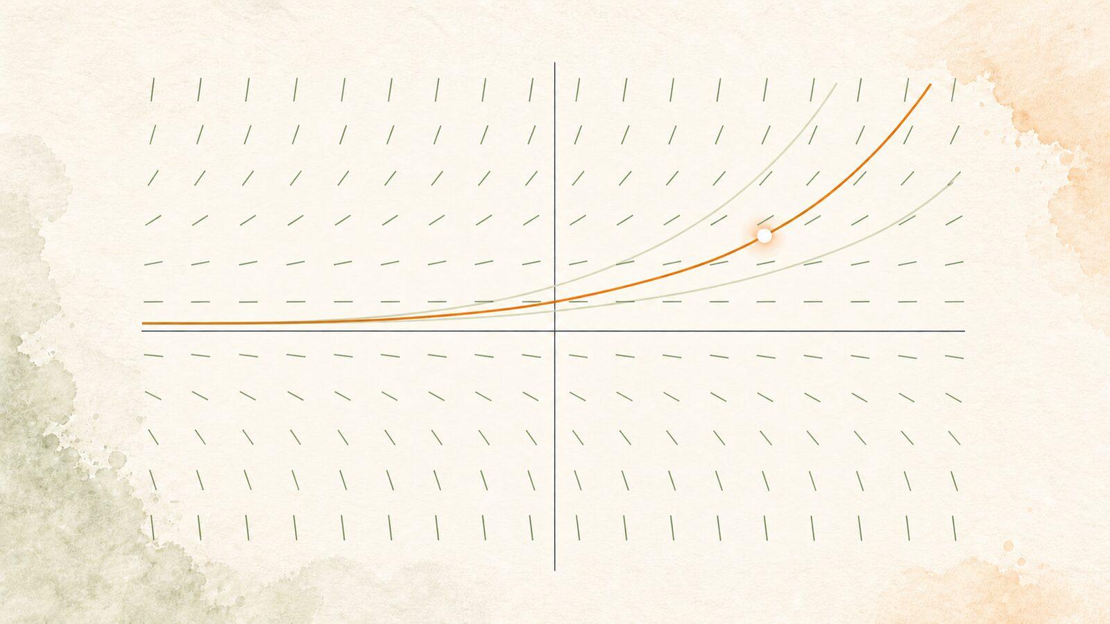
The picture that makes explicit first-order differential equations readable is a field of tiny slopes. For an equation written y' = F(x, y), every point where F is defined receives a short segment telling a curve which way to lean. A solution is a path that follows those directions. Once you see that field, solution families, initial conditions, and exponential growth stop looking like separate tricks.

A Differential Equation Is a Rule for Change

A derivative tells you how fast a quantity is changing. A differential equation turns that idea around. It gives you a relationship involving the derivative and asks you to recover the quantity.

Consider

$$y' = 2y$$

The prime means the derivative of y with respect to x. The equation says that the rate of change is always twice the current value. When y is 1, the slope must be 2. When y is 3, the slope must be 6. When y is negative, the slope must be negative. The rule does not directly tell you the height of the curve at any particular x. It tells you how the height and the slope must travel together.

This is the central reversal:

• In calculus, you know the function and compute its rate of change.
• In a differential equation, you know a rule for the rate of change and reconstruct the function.

The equation y' = 2y is first order because its highest derivative is the first derivative. An equation involving y'' is second order. The word order tells you how many layers of change the rule reaches, not how difficult the equation looks.

It is also an ordinary differential equation, or ODE, because y depends on one independent variable. If a temperature depends on both position and time, its model uses partial derivatives and becomes a partial differential equation, or PDE. The same big idea survives, but this article stays with ODEs: one input, one evolving path.

The Solution Is a Function, Not a Number

To solve y' = 2y, you need a function whose derivative is twice itself. Exponential functions have exactly that behavior. Try

$$y = Ce^{2x}$$

where C is any constant. Differentiate it:

$$y' = 2Ce^{2x}$$

Since y itself is $Ce^{2x}$, this says y' = 2y. The proposed function satisfies the equation at every x, so it is a solution.

Notice what verification looks like. With an algebraic equation, you substitute a number. With a differential equation, you differentiate a function and substitute the result. A correct solution has to obey the rule everywhere on the interval you are considering, not merely pass through one convenient point.

The constant C is not unfinished work. It is part of the answer. The equation describes a family of curves:

• $C = 1$ gives $y = e^{2x}$.
• $C = 3$ gives $y = 3e^{2x}$.
• $C = -2$ gives $y = -2e^{2x}$.
• C = 0 gives the flat solution y = 0.

Every member has the same growth rule, but each starts at a different height. A law of change cannot tell you where the story began. That missing starting information is exactly what the constant stores.

This is also why integration introduces an additive constant. Differentiation erases constant vertical shifts because their derivative is zero, so reversing the process must keep every possible shift. Later algebra may change how that parameter looks. In this example, exponentiating turns $e^{C}$ into a multiplicative constant in front of $e^{2x}$.

Slope Fields Turn the Rule Into a Landscape

You can understand an explicit first-order equation y' = F(x, y) before solving it symbolically. Take a grid of points where F is defined. At each one, calculate the required slope, then draw a short line segment with that slope. The result is called a slope field or direction field.

For y' = 2y, the slope depends only on height:

• Along y = 0, every segment is horizontal.
• Along y = 1, every segment has slope 2.
• Along y = -1, every segment has slope -2.
• Higher positive rows tilt upward more sharply.
• Lower negative rows tilt downward more sharply.

The field looks like horizontal bands of equal tilt. A solution curve can start at any point, but after that it must follow the local segments. Positive solutions bend upward and grow. Negative solutions fall away from zero. The zero solution stays flat because every arrow on that line is horizontal.

This picture separates the equation from any one solution. The differential equation creates the whole field. Each solution is one thread through it.

It also lets you predict behavior without finding a formula. If the segments point upward in a region, solutions increase there. If they are horizontal along y = c for every relevant x, then y = c is a constant equilibrium solution. If nearby segments point toward that line, nearby solutions are pulled back toward it. If they point away, small disturbances grow. Much of applied differential equations is this kind of qualitative reading: understand what paths can do before deriving their exact formulas.

For y' = 2y, the right-hand side changes smoothly with y, so the standard existence-and-uniqueness conditions guarantee one solution through each point. The slope field illustrates that result, but it does not prove it. Sharing a point and slope is not enough for every equation: less regular rules can allow solutions to meet and later separate.

Initial Conditions Pick One Path

Now add the condition y(0) = 3 to the same equation. This is an initial condition: at x = 0, the curve passes through height 3. Start with the solution family

$$y = Ce^{2x}$$

and substitute the known point:

$$3 = Ce^{0} = C$$

so the particular solution is

$$y = 3e^{2x}$$

The differential equation supplied the shape of the family. The initial condition selected one member. In the slope-field picture, it placed your finger at the point (0, 3), leaving only the path through that point.

For regular initial-value problems, the number of conditions you normally need tracks the order of the equation. A first-order velocity law y' = v(x, y), where the velocity is already specified, usually needs one initial position. A second-order acceleration law generally needs both an initial position and an initial velocity.

For example, the normalized undamped spring equation

$$y'' + y = 0$$

says that acceleration points back toward equilibrium. The physical form is m y'' + k y = 0; choosing units with k/m = 1 produces the normalized equation above. Its solutions combine sine and cosine. Knowing only the starting position does not tell you whether the spring was released from rest or already moving. Add the starting velocity, and the motion becomes determined.

Separation of Variables Means Undoing the Link

The equation y' = 2y can be solved systematically, not just guessed. Write the derivative as $\frac{dy}{dx}$:

$$\frac{dy}{dx} = 2y$$

Move the y part beside dy and the x part beside dx:

$$\frac{dy}{y} = 2 dx$$

Now integrate both sides:

$$\ln|y| = 2x + C$$

Exponentiating gives

$$y = Ae^{2x}$$

where A is nonzero at this stage because dividing by y excluded y = 0. Test the excluded function in the original equation: y = 0 works. The complete family can therefore be written y = $Ae^{2x}$ for any real constant A, including zero.

The method is called separation of variables because it separates everything involving y from everything involving x before integrating. It works for equations that can be rearranged into the form

$$\frac{dy}{dx} = f(x)g(y)$$

but the algebra carries a trap. Dividing by g(y) can discard solutions where g(y) = 0. In the example, dividing by y temporarily excluded the equilibrium y = 0.

For the smooth equations normally introduced with separation, restoring excluded equilibria completes the family. Less regular equations can also have piecewise solutions that wait at an equilibrium before leaving, so separation is not a universal completeness proof. After dividing or rearranging, test the derived family and every excluded value against the original equation.

Growth, Decay, and Oscillation Are Different Rules

Small changes in a differential equation produce very different kinds of motion.

The model

$$y' = ky$$

models exponential growth for positive quantities when k is positive and exponential decay toward zero when k is negative. More generally, the magnitude of any nonzero solution grows for positive k and shrinks for negative k. The model appears whenever the rate is proportional to the current amount: idealized population growth, continuously compounded money, and radioactive decay are familiar examples. The same formula does not make every real population or investment exponential forever. It says that exponential behavior follows if the proportional-rate assumption remains true.

The spring equation y'' + y = 0 produces oscillation instead. Its solutions are built from sine and cosine because differentiating twice reverses their sign. Compare it with

$$y'' - y = 0$$

whose solutions are built from exponentials, or equivalently from hyperbolic functions. The sign determines whether the system is pulled back into repeated motion or pushed into growth and decay.

Real models add terms for outside forces, friction, limited resources, or interactions among several quantities. A logistic population model slows growth near a carrying capacity. A damped spring loses amplitude over time. A system of differential equations can track several quantities changing together. Each added term changes the local rule, and therefore which paths the system can follow.

Where the Mistakes Come From

The first mistake is searching for a number. In a differential equation, the unknown is usually a function. If your answer is one value of y without a requested evaluation point, you probably stopped too soon.

The second is checking only an initial condition. Passing through (0, 3) does not make a curve a solution of y' = 2y. Infinitely many curves pass through that point. The curve must also satisfy the derivative rule throughout the interval.

The third is dropping the arbitrary constant. A differential equation without enough conditions normally describes a family. Writing one member as if it were the whole answer throws away valid histories.

The fourth is losing an equilibrium while dividing. If you divide by y, y - 1, or any expression involving the unknown function, stop and test the zero values of that expression in the original equation.

The fifth is treating a model as the thing itself. y' = ky produces exponential growth or decay because it assumes a constant proportional rate. A real system follows that curve only while the assumption is a useful approximation. Solving the equation correctly does not prove that the equation was the right model.

Where Math Zen Fits In

Differential equations combine several skills that are often learned in separate chapters. You need to read a derivative as a rate, rearrange algebra without losing cases, recognize when an exponential differentiates into itself, integrate both sides, and use an initial condition to determine the remaining constant. A weakness in any one layer can make the whole method feel mysterious.

Math Zen includes practice with separable, first-order linear, second-order, homogeneous, exact, Bernoulli, and systems of ordinary differential equations. Before calculating, use the same three questions from this article: what change does the equation require, what family of paths could obey it, and which conditions select the path you need?

The useful practice loop is simple: classify one equation, predict the direction of its solutions, solve or verify it, then check the initial condition and any excluded equilibria. Return to the mix after a gap, following the same spaced-repetition approach used across the rest of Math Zen. The goal is not to memorize a shelf of recipes. It is to see which rule for change is in front of you.

The Bottom Line

A differential equation describes a relationship between a quantity and the way it changes. Its solution is an entire function, often one member of a family. The arbitrary constant records where the path could have started, and an initial condition chooses the path that matches the actual starting point.

For explicit first-order equations, the slope-field picture holds the subject together. The local rule fills its domain with permitted directions, and a solution follows them. Separation of variables, initial-value problems, growth, decay, and oscillation are different ways of reading or tracing that landscape. A differential equation turns a local rule for change into a global curve.