Understanding Laplace Transforms Intuitively (Calculus into Algebra)

Solving a differential equation by hand can feel like walking through thick mud. In our differential equations post, we saw that solving an equation means finding an entire function whose rates of change satisfy a local rule. For basic first-order equations, separating variables works smoothly. But add a second derivative, an external driving force, a sudden voltage switch, or a physical shock, and classical calculus methods quickly become tangled in chains of integration by parts, undetermined coefficients, and systems of constants.

Then engineering textbooks introduce an unexpected escape hatch. They take the difficult differential equation, multiply it by an exponential, integrate from zero to infinity, and suddenly all the derivatives vanish. In their place stands an ordinary high school polynomial equation. You solve for the unknown using basic division, look up the answer in a reference table, and the problem is finished.

This machinery is the Laplace transform. To most students meeting it for the first time, it looks like black magic: an arbitrary recipe that somehow bypasses the hardest parts of calculus. This guide provides the bridge between the mechanical formula and the intuition behind it. The Laplace transform is not a trick; it is a change of perspective from time to frequency, and every step of the process is an operation you already understand.

The Language Exchange: Turning Calculus into Algebra

The best analogy for an integral transform comes from language translation. Imagine you are working on a crossword puzzle written in English, and you come across a clue about an obscure medical plant native to South America. You do not know the answer, but you have a botanist friend who knows the subject intimately. The catch is that your friend speaks only Spanish.

You do not abandon the puzzle. Instead, you translate the clue into Spanish, phone your friend, and receive the one-word answer in Spanish. Then you translate that single word back into English and write it in your crossword grid. Even with two rounds of translation, this indirect route is vastly easier than spending three years studying botany yourself.

The Laplace transform performs exactly this language exchange for mathematics:

• The Time Domain (English): This is where physical problems live. You have masses bouncing on springs, currents flowing through resistors and capacitors, or populations fluctuating. The laws of physics are written in rates of change, which means derivatives, integrals, and differential equations.
• The S-Domain (Spanish): This is the transformed algebraic realm. In this world, the independent variable is s rather than time t. Most importantly, calculus does not exist here. Rates of change become ordinary multiplication, and accumulating history becomes ordinary division.
• The Translation Table (Dictionary): Instead of solving the differential equation in the time domain, you translate it into the s-domain. You solve the resulting equation using elementary high school algebra. Once you have isolated your unknown, you look up the algebraic expression in your transform table to translate it back into time.

What looks like extra work, transforming into a new space only to transform back, is actually the ultimate shortcut. Algebra is systematically easier than calculus, and the Laplace transform lets algebra do the heavy lifting.

The S-Domain as a Decay and Frequency Dial

To understand how this translation occurs, look at the variable s. In introductory calculus, functions depend on real numbers like time t or position x. In the Laplace transform, the transformed function F(s) depends on a complex variable s.

Think of s as a tuning dial with two independent knobs:

$$s = \sigma + i\omega$$

The real part, σ, controls exponential growth or decay. It tells you how rapidly a signal fades away or blows up over time. As we explored in the exponents post, $e^{\sigma t}$ is the fundamental currency of continuous compounding.

The imaginary part, ω, controls pure oscillation. It is the frequency dial, determining how many times per second a sine wave cycles. The imaginary unit i is a rotation operator, spinning numbers around a circle rather than sliding them along a line.

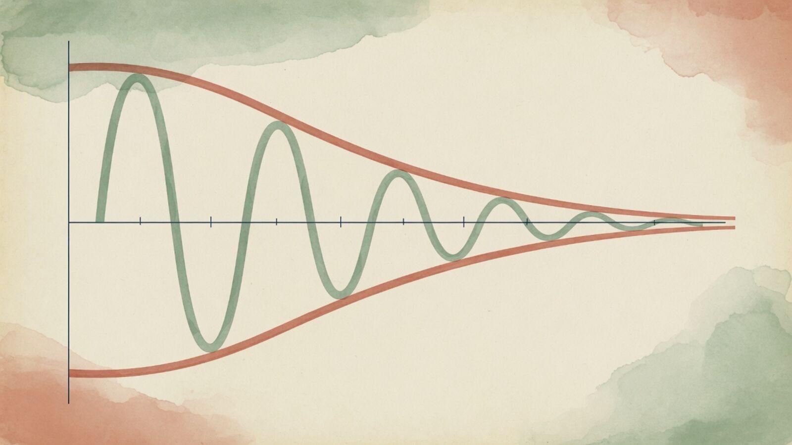
When you combine both knobs into $e^{-st}$, you get an exponential wave that oscillates while decaying toward zero. The variable s is not an abstract placeholder; it is a coordinate system that describes building blocks. Every physical motion you care about, steady states, fading vibrations, exponential growth, resonance, can be constructed by combining these decaying oscillatory components.

The Kernel Integral: Testing Functions Against Exponentials

The mathematical machine that translates a time function f(t) into the s-domain is an improper integral:

$$L[f(t)] = F(s) = \int_0^{\infty} f(t)\, e^{-st}\, dt$$

This looks intimidating, but its mechanism is straightforward. It is a continuous correlation detector, or a resonance test.

Take your time function f(t), which describes whatever your system is doing from time t = 0 forward. Now choose a specific test frequency and decay rate on your dial, setting s. You multiply your function by $e^{-st}$ and add up the area under the product from zero to infinity.

If your function f(t) contains nothing that matches your chosen s, the positive and negative oscillations cancel each other out, or the heavy decay squashes the product to near zero. The total integral is small. But if your function naturally contains an oscillation or decay that resonates with that s, the product reinforces itself, and the integral accumulates a large value.

The resulting function F(s) is a map of resonance. It evaluates every possible value of s and records how strongly your original time signal rings at that specific combination of frequency and decay. You have converted a timeline into a frequency spectrum.

Why start the integral at t = 0? Because physical systems have a start time. You flip a switch, strike a bell, or release a pendulum at t = 0. The unilateral Laplace transform is tailored specifically for cause-and-effect systems where what happened before the start is either zero or wrapped entirely into your initial conditions.

Turning Derivatives into Multiplication

Now we arrive at the core superpower of the Laplace transform. Why does this integral transform derivatives into elementary algebra?

The answer lies in integration by parts. Suppose you want to compute the Laplace transform of a derivative, y'(t). By definition:

$$L[y'(t)] = \int_0^{\infty} y'(t)\, e^{-st}\, dt$$

Recall the integration by parts rule: $\int u\, dv = uv - \int v\, du$. Let $u = e^{-st}$ and $dv = y'(t)\, dt$. That means $du = -s e^{-st}\, dt$ and $v = y(t)$.

Substitute these parts into the integral:

$$L[y'(t)] = \bigl[y(t)\, e^{-st}\bigr]_0^{\infty} - \int_0^{\infty} y(t)\,(-s e^{-st})\, dt$$

Evaluate the boundary term $\bigl[y(t)\, e^{-st}\bigr]$ from 0 to infinity. At infinity, assuming s has a large enough real part to overpower y(t), the term $e^{-st}$ crushes the expression to zero. At t = 0, $e^{0}$ is 1, leaving -y(0).

Now look at the remaining integral. The factor -s is a constant with respect to time t, so you can pull it out front. Two minus signs make a plus:

$$\int_0^{\infty} y(t)\,(-s e^{-st})\, dt = -s \int_0^{\infty} y(t)\, e^{-st}\, dt$$

Notice what that remaining integral is: it is the exact definition of L[y(t)], or Y(s). Putting the pieces together gives the famous identity:

$$L[y'(t)] = s Y(s) - y(0)$$

Look closely at what just happened. Taking the derivative of y(t) in the time domain turned into multiplying Y(s) by s in the frequency domain, with a subtraction for the starting value y(0).

Repeat the exact same integration by parts for a second derivative, y''(t), and you find:

$$L[y''(t)] = s^2 Y(s) - s y(0) - y'(0)$$

Differentiating twice becomes multiplying by $s^2$. Differentiating three times becomes multiplying by $s^3$. The fundamental operation of calculus, differentiation, which requires limits and delicate infinitesimal ratios, has been converted into ordinary grade school multiplication.

Initial Conditions Are Built In, Not Added Later

In classical differential equations, solving an initial value problem is a two-phase chore:

1. You ignore the initial conditions and spend several pages finding the general solution, dragging along arbitrary constants C₁ and C₂.
2. Once you have the general formula, you differentiate it, substitute t = 0, set up a linear system of equations for C₁ and C₂, and solve for the specific constants.

If you make an algebra error in phase one, all of phase two is ruined.

The Laplace transform eliminates this two-step dance. Look again at the transform of the derivatives:

$$L[y'(t)] = s Y(s) - y(0)$$ $$L[y''(t)] = s^2 Y(s) - s y(0) - y'(0)$$

The initial values y(0) and y'(0) are baked directly into the algebraic translation. They appear on line one of your calculation as known numbers.

Consider a simple harmonic oscillator, such as a mass on a spring starting from rest with an initial displacement of 3 units:

$$y'' + 4y = 0, \quad y(0) = 3,\ y'(0) = 0$$

Transform the entire equation into the s-domain term by term:

$$(s^2 Y(s) - s y(0) - y'(0)) + 4 Y(s) = 0$$

Substitute the known initial numbers y(0) = 3 and y'(0) = 0:

$$(s^2 Y(s) - 3s) + 4 Y(s) = 0$$

Group the Y(s) terms:

$$(s^2 + 4) Y(s) - 3s = 0$$

Add 3s to both sides and divide:

$Y(s) = \frac{3s}{s^2 + 4}$

In four lines of elementary algebra, the differential equation is completely solved in the s-domain. There are no undetermined constants C to find, and no second phase of work. The specific answer for those exact initial conditions is sitting right in front of you.

The Return Journey: Inverses and Partial Fractions

We now have the solution in the s-domain: $Y(s) = \frac{3s}{s^2 + 4}$. But an engineer cannot build a physical circuit or damp a physical bridge using s-domain coordinates; we live in time t. We must translate the answer back.

Mathematically, the inverse Laplace transform is defined by a complex contour integral along a vertical line in the complex plane, known as the Bromwich integral. In practice, almost nobody evaluates this contour integral for standard problems. Instead, we use partial fraction decomposition and standard tables.

From any standard table of Laplace transform pairs, you find two foundational entries:

• $L[\cos(\omega t)] = \frac{s}{s^2 + \omega^2}$
• $L[\sin(\omega t)] = \frac{\omega}{s^2 + \omega^2}$

Compare our solved algebraic expression, $Y(s) = 3 \frac{s}{s^2 + 2^2}$, with the cosine transform where ω = 2. The match is immediate:

$$y(t) = 3\cos(2t)$$

The problem is solved. The oscillation has an amplitude of 3 and an angular frequency of 2 radians per second, satisfying both the differential equation and the initial conditions.

When solving more complex systems, the denominator of Y(s) will often be a high-degree polynomial, such as $(s-1)(s+2)(s^2+9)$. In those cases, partial fractions break the single tangled fraction into a sum of simple terms:

$$\dfrac{A}{s-1} + \dfrac{B}{s+2} + \dfrac{Cs + D}{s^2 + 9}$$

Because the Laplace transform is linear, each simple fraction translates back into its own recognizable time behavior:

• $\frac{A}{s-1}$ becomes an exponential growth term: $A e^{t}$
• $\frac{B}{s+2}$ becomes an exponential decay term: $B e^{-2t}$
• $\frac{Cs + D}{s^2 + 9}$ becomes a combination of sine and cosine oscillating at frequency 3

Partial fractions are simply the act of unmixing the frequencies, sorting the complex frequency response back into its individual physical voices.

Where the Mistakes Come From

Students working with Laplace transforms encounter errors in three predictable places. Understanding these failure modes preserves the intuitive clarity of the method.

The first mistake is sign confusion with initial conditions. In the derivative formula, the initial values carry negative signs: $L[y'] = s Y(s) - y(0)$. When y(0) is itself a negative number, such as y(0) = -5, students frequently write $s Y(s) - 5$ instead of $s Y(s) - (-5) = s Y(s) + 5$. When moved across the equals sign to isolate Y(s), the sign flips again. Always write the formula with explicit parentheses before plugging in negative initial conditions.

The second mistake is variable bleed, mixing t and s in the same expression. The Laplace transform is an all-or-nothing bridge. Once you apply the integral operator, every t must be integrated out; no t may remain in the s-domain. Conversely, when taking the inverse transform, no s may linger in your final time equation. If you find yourself writing st, stop immediately; an operator was applied incompletely.

The third mistake is treating table lookups as rote pattern matching without completing the square. When an s-domain denominator cannot be factored over real numbers, such as $s^2 + 6s + 13$, students often stall. Completing the square rewrites it as $(s + 3)^2 + 4$, which immediately reveals a shifted sine or cosine: an oscillation at frequency 2 damped by an exponential envelope $e^{-3t}$. The algebra is not an obstacle to the physics; it is revealing the physical behavior.

Where Math Zen Fits In

The Laplace transform shifts the difficulty of differential equations entirely onto algebraic execution. You never have to evaluate painful integrals during the problem, but in exchange, your algebra must be spotless.

If your partial fraction decomposition is shaky, your sign arithmetic slips on initial values, or completing the square takes three minutes of hesitation, the method breaks down. Math Zen is designed to make those foundational building blocks second nature:

• Polynomial Division and Factoring: Speed drills for decomposing denominators into linear and irreducible quadratic factors without hesitation.
• Partial Fraction Expansion: Targeted practice solving for numerators using both the cover-up method and system equating.
• Exponential and Complex Number Fluency: Developing immediate reflex for the relationship between real decay rates, imaginary frequencies, and sinusoidal behavior.

By drilling these component skills in short, focused daily sessions, you build the computational stamina that makes advanced methods effortless. Once the algebra is automatic, solving differential equations with the Laplace transforms practice module becomes straightforward pattern recognition.

The Bottom Line

The Laplace transform is not an exotic trick created to torment engineering students. It is a change of coordinates from time to frequency that turns the calculus of change into the algebra of arithmetic.

The kernel $e^{-st}$ acts as a resonance probe, testing a time signal against decaying oscillations. Integration by parts ensures that differentiating in time becomes multiplying by s in frequency. Initial conditions are incorporated from line one rather than patched in at the end. And partial fractions untangle the resulting algebraic solution so that reference tables can carry you back to the time domain.

When a problem in time looks like an impenetrable maze, do not fight the calculus head-on. Step sideways into the s-domain, let simple algebra find the path, and step back into time with the solution in hand.