Understanding Eigenvalues Intuitively (The Directions a Matrix Leaves Alone)

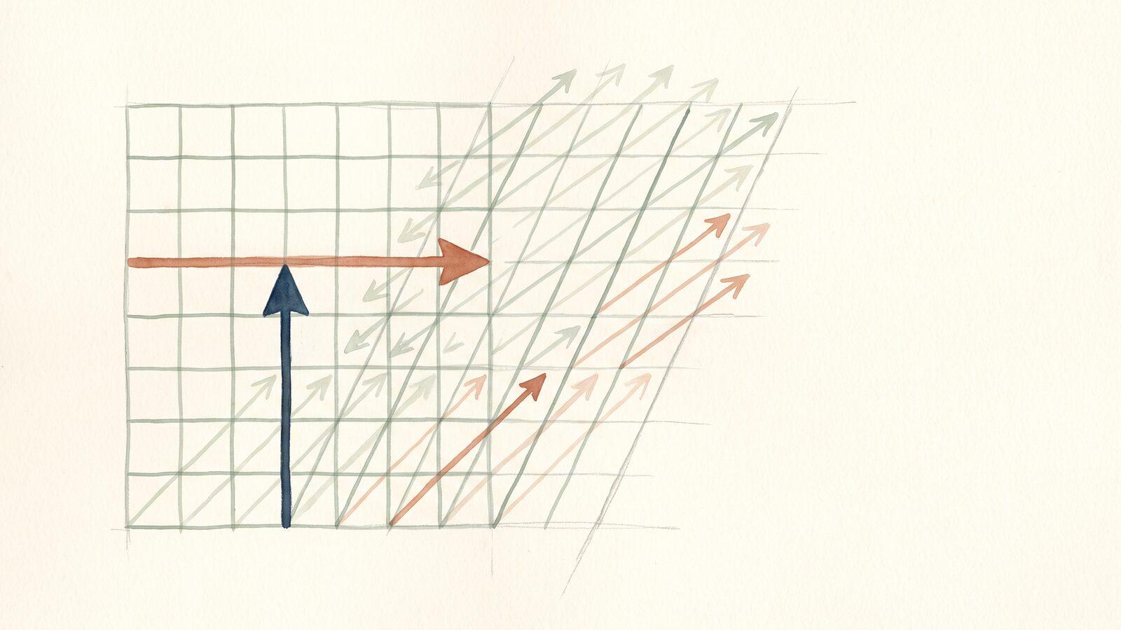
Put a sheet of rubber on a table, draw a hundred short arrows on it in every direction, and pull the sheet so that it stretches sideways twice as far as it stretches up. Watch the arrows. Almost all of them swing toward the horizontal as the sheet deforms. Two of them do not move at all. The arrow that was already horizontal stays horizontal and gets twice as long. The arrow that was vertical stays vertical and keeps its length.

Those two arrows are the eigenvectors of the stretch, and the numbers 2 and 1 are its eigenvalues. Everything in this topic, the formula with the determinant, the characteristic polynomial, diagonalization, the complex numbers that show up when a matrix rotates, is a way of finding those special arrows for a machine you cannot see by looking.

If you have not read Understanding Matrices Intuitively, this is the sequel. That article set up the picture of a matrix as a machine that takes a trip and returns a trip. This one asks the machine a single question: which trips do you leave alone?

A Matrix Is a Machine, and Most Arrows Get Turned

A matrix $A$ takes a vector $\vec{v}$ and produces a new vector $A\vec{v}$. For most inputs, the output points somewhere new. A shear tilts arrows. A rotation swings every arrow by the same angle. A stretch that is stronger in one direction than another drags arrows toward the direction of the stronger pull.

Think of the matrix as a wind tunnel. Arrows go in, wind hits them, and they come out bent. The interesting question is not what happens to a typical arrow. It is whether there is any arrow the wind cannot bend, an arrow that comes out pointing exactly the way it went in, merely longer or shorter.

The Arrows That Refuse to Turn

An eigenvector of $A$ is a nonzero vector $\vec{v}$ that the machine keeps on its own line:

$$A\vec{v} = \lambda\vec{v}$$

The Greek letter lambda, $\lambda$, is the eigenvalue: the factor the arrow was scaled by. The equation says the machine acting on this particular arrow is indistinguishable from plain multiplication by a number. Along an eigenvector, the matrix stops being a matrix and becomes a scalar.

The eigenvalue carries a lot of information in one number:

• $\lambda > 1$ means the machine lengthens that direction.
• $0 < \lambda < 1$ means it shortens it.
• $\lambda = 1$ means it leaves that direction completely untouched.
• $\lambda < 0$ means it flips the arrow to point the opposite way, then scales it.
• $\lambda = 0$ means it crushes that direction to nothing. The machine flattens space along that line.

Note what an eigenvector is not. It is not a single arrow but a direction: if $\vec{v}$ is an eigenvector then so is $3\vec{v}$, with the same eigenvalue. And the zero vector is excluded by definition, because every matrix sends zero to zero, which would make every number an eigenvalue and the whole idea useless.

Where the Formula Comes From

Textbooks hand you $\det(A - \lambda I) = 0$ as if it fell from the sky. It comes from the sentence above.

Start with $A\vec{v} = \lambda\vec{v}$. The right side is a number times a vector. To move it across the equals sign you need it in matrix form, and $\lambda\vec{v}$ is the same as $\lambda I\vec{v}$, where $I$ is the identity matrix that does nothing. Now subtract:

$$(A - \lambda I)\vec{v} = \vec{0}$$

Read this as a statement about a new machine, $A - \lambda I$. It takes a nonzero arrow $\vec{v}$ and returns the zero vector. A machine that sends a real arrow to a point has flattened at least one direction of space. In the matrix article we saw that the determinant measures how much area survives a machine, so a machine that flattens has determinant zero:

$$\det(A - \lambda I) = 0$$

That is the whole derivation. The eigenvalues are the values of $\lambda$ that break the machine $A - \lambda I$, and the eigenvectors are the directions it breaks along. Expanding the determinant gives a polynomial in $\lambda$, called the characteristic polynomial, and its roots are the eigenvalues. For a $2 \times 2$ matrix it is a quadratic; for $n \times n$ it has degree $n$, which is why an $n \times n$ matrix has at most $n$ eigenvalues.

A Worked Example, Slowly

Take the matrix

$$A = \begin{pmatrix} 2 & 1 \\ 1 & 2 \end{pmatrix}$$

Subtract $\lambda$ down the diagonal and take the determinant:

$$\det\begin{pmatrix} 2 - \lambda & 1 \\ 1 & 2 - \lambda \end{pmatrix} = (2 - \lambda)^2 - 1 = \lambda^2 - 4\lambda + 3$$

Set it to zero and factor: $(\lambda - 3)(\lambda - 1) = 0$, so the eigenvalues are $\lambda = 3$ and $\lambda = 1$.

Now find the direction for each. For $\lambda = 3$, solve $(A - 3I)\vec{v} = \vec{0}$:

$$\begin{pmatrix} -1 & 1 \\ 1 & -1 \end{pmatrix}\begin{pmatrix} x \\ y \end{pmatrix} = \begin{pmatrix} 0 \\ 0 \end{pmatrix}$$

Both rows say $x = y$, so the eigenvector is any multiple of $(1, 1)$. Check it against the original machine: $A(1,1) = (3, 3) = 3 \cdot (1, 1)$. The diagonal arrow comes out three times longer, pointing the same way.

For $\lambda = 1$ the rows say $x = -y$, so the eigenvector is any multiple of $(1, -1)$, and indeed $A(1,-1) = (1,-1)$. The anti-diagonal arrow is untouched.

Now you can describe this matrix in a sentence, which you could not do from its four entries: it stretches space by a factor of 3 along the diagonal and leaves the anti-diagonal alone. Every other arrow in the plane gets dragged toward the diagonal, because the diagonal component grows three times faster than the other one.

What the Eigenvalues Tell You About the Machine

Two facts fall out of the characteristic polynomial and are worth keeping.

The product of the eigenvalues is the determinant. In the example, $3 \times 1 = 3$, and the determinant of $A$ is $2 \cdot 2 - 1 \cdot 1 = 3$. This makes sense: the determinant is the area scaling of the whole machine, and if the machine stretches by 3 along one direction and 1 along another, area scales by 3.

The sum of the eigenvalues is the trace, the sum of the diagonal entries. Here $3 + 1 = 4 = 2 + 2$. Both facts are quick checks that your arithmetic survived.

More broadly, the eigenvalues are a spectrum of the machine. Large ones are the directions that dominate after the machine is applied many times. A machine with eigenvalues $3$ and $1$, applied ten times, stretches its first eigenvector by $3^{10}$ and its second by $1$. Any starting arrow with even a trace of the first direction ends up almost perfectly aligned with it. This is why repeated processes settle into an eigenvector: it is the direction that wins.

Complex Eigenvalues Mean Rotation

Rotate the plane by 90 degrees. Every arrow turns. No direction is left alone, so there should be no eigenvectors, and the formula agrees. The rotation matrix is

$$R = \begin{pmatrix} 0 & -1 \\ 1 & 0 \end{pmatrix}$$

and its characteristic polynomial is $\lambda^2 + 1 = 0$, which has no real solutions. Its eigenvalues are $i$ and $-i$.

This is not a failure of the method. It is the method telling you something true: this machine rotates, and rotation has no fixed direction in the real plane. A complex eigenvalue is the signature of a twist. A general rotation by angle $\theta$ has eigenvalues $e^{i\theta}$ and $e^{-i\theta}$, the same rotating numbers from Euler's identity, and a matrix with eigenvalues like $0.9 e^{\pm i\theta}$ spirals inward, rotating and shrinking at once. If complex numbers still feel like a trick, Understanding Imaginary Numbers Intuitively builds the picture of $i$ as a quarter turn, which is exactly the role it plays here.

Diagonalization: Change Seats and the Machine Becomes Multiplication

Suppose an $n \times n$ matrix has $n$ eigenvectors that point in genuinely different directions. Then those eigenvectors can serve as a new set of axes. Describe every vector in terms of how much of each eigenvector it contains, and the machine becomes trivial: it just multiplies each coordinate by the matching eigenvalue.

Written out, if $P$ is the matrix whose columns are the eigenvectors and $D$ is the diagonal matrix of eigenvalues, then

$$A = P D P^{-1}$$

Read it right to left. $P^{-1}$ translates a vector into eigenvector coordinates, $D$ scales each coordinate, and $P$ translates back. The machine has not changed. You have found the seats from which it looks like a list of numbers.

The payoff is powers. Applying the machine a hundred times means

$$A^{100} = P D^{100} P^{-1}$$

and $D^{100}$ is just each eigenvalue raised to the hundredth power. A calculation that would take a hundred matrix multiplications becomes a handful of scalar ones. Every long-run question about a matrix, what a population does after fifty generations, what a random walk converges to, how a vibration decays, is a question about $D^n$.

Why Everything Hunts for Eigenvectors

Once you see eigenvectors as the directions that win under repetition, the applications stop looking like a list and start looking like one idea.

• PageRank. Google's original ranking is the eigenvector, with eigenvalue 1, of a giant matrix describing which pages link to which. It is the distribution of attention that stays put when you follow links one more time.
• Differential equations. A system $\dot{\vec{x}} = A\vec{x}$ has solutions built from $e^{\lambda t}$ along each eigenvector. Positive eigenvalues grow, negative ones decay, complex ones oscillate. The eigenvalues are the rates of the system. Laplace transforms are the same hunt for exponential behavior, carried out with an integral instead of a determinant.
• Vibrations. A bridge, a guitar string, or a molecule has natural frequencies, and they are the eigenvalues of its stiffness matrix. The eigenvectors are the shapes it vibrates in.
• Data. Principal component analysis finds the eigenvectors of a covariance matrix. The eigenvector with the largest eigenvalue is the direction along which the data varies most, which is the first axis you would choose to summarize it.
• Quantum mechanics. Observable quantities are eigenvalues of operators. A measurement returns one of the eigenvalues, and the eigenvectors are the states the system settles into.

In each case the method is the same: find the directions the machine leaves alone, and the complicated behavior becomes multiplication along those directions.

Where the Mistakes Come From

The errors in this topic are consistent, and most of them come from losing the picture.

Accepting the zero vector. Solving $(A - \lambda I)\vec{v} = \vec{0}$ always allows $\vec{v} = \vec{0}$. That is not an eigenvector. If your only solution is zero, you used the wrong $\lambda$.

Expecting one row to give the answer. In the worked example, both rows of $(A - \lambda I)$ said the same thing, $x = y$. That redundancy is not a mistake; it is the flattening. If both rows give independent equations with only the zero solution, the eigenvalue is wrong.

Assuming there are always enough eigenvectors. The shear matrix with rows $(1, 1)$ and $(0, 1)$ has the single eigenvalue $1$, repeated, but only one eigenvector direction. It cannot be diagonalized. Repeated eigenvalues are where you check rather than assume.

Confusing the two words. An eigenvalue is a number. An eigenvector is a direction. Questions that ask for one usually need the other as a step, and answers that hand back the wrong kind of object are the most common way to lose the mark.

Sign slips in the characteristic polynomial. For a $2 \times 2$ matrix the polynomial is always $\lambda^2 - (\text{trace})\lambda + \det$. Writing it that way, and checking that the roots multiply to the determinant, catches most slips.

Normalizing when nobody asked. An eigenvector is any nonzero vector on its line. Scaling it to length 1 is sometimes required and often optional; do it only when the question says so, and never lose the direction while doing it.

Where Math Zen Fits In

The picture of a machine stretching some directions and turning others is worth an hour of staring. The mechanics, subtracting $\lambda$ down the diagonal, expanding the determinant, factoring, back-substituting to get the direction, are worth thirty problems, because every one of the mistakes above is a habit that only repetition breaks.

The Matrices topic in Math Zen generates fresh eigenvalue problems with the answer checked against your work, from $2 \times 2$ characteristic polynomials through eigenvectors and the trace and determinant checks, alongside the determinants and inverses they depend on. The explanation next to each problem shows the flattening picture, not just the algebra, so the formula stays attached to the reason it works.

The Bottom Line

A matrix turns most arrows. An eigenvector is an arrow it does not turn, and the eigenvalue is how much it stretches that arrow instead. The formula $\det(A - \lambda I) = 0$ is just the observation that $A - \lambda I$ must flatten space along an eigenvector, and a flattened machine has determinant zero. Complex eigenvalues mean the machine rotates, diagonalization means describing the machine from the seats where it looks like plain multiplication, and repeated processes end up along the eigenvector with the largest eigenvalue, which is why search engines, bridges, and populations all come down to the same calculation.

Find the directions the machine leaves alone, and the machine stops being mysterious.